Motivation

The solar energy industry has had an average annual growth rate of 59% over the last 10 years.  Prices have dropped 52% over last 5 years and last year, solar accounted for 30% of all new capacity installed*. So things are going pretty well. The challenge, however, is that solar power is variable – the sun don’t shine all the time, not even in California! We can store solar energy in a battery and release it to meet consumption or sell it on to the grid or to peers.

 

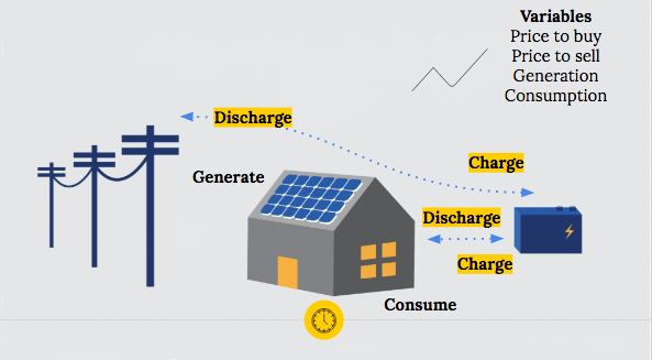
The set-up is that there is a commercial building with photovoltaic panels and a battery. The building can use the energy from the grid, the photovoltaic panels or the battery to meet its energy needs.  Since the generation, consumption and the prices to buy or sell vary throughout the day, the composition of energy use and when to charge and discharge the battery is strategic according to how expensive energy is during that time period.

Goal

So the goal of this project was to be able to save the most money spent on energy over a period of 10 days whilst being able to meet all the energy needs of the building and not going outside the physical constraints of the battery. I used data from Schneider Electric, a European company specialised in energy management (as part of a Driven Data competition). I had the day ahead prices, and previous consumption and generation data for 11 commercial sites for 10 periods of 10 days. The concrete output was a suggested level of charge every 15 mins for each building.

Process

So my process was forecasting day ahead consumption and generation for each site, and then feeding this into a reinforcement learning process. My final success metric which I was optimising for was what percentage of money I saved through deploying this optimiser compared with meeting the energy needs of the building solely from the grid.

Forecasting

I forecast energy consumption using traditional time series methods such as AR, ARMA and ARIMA with machine learning approaches such as gradient boosting and an LSTM neural network. I engineered features to do with the time e.g. hourly, daily, weekly, monthly and seasonally. I controlled for the site but anticipate that the models would have benefitted from additional information about the site, and what the electricity was being used for, but the company didn’t provide this information.  Knowing the location of the site would also have allowed me to forecast energy generation with more accurate radiance data. (I did not forecast energy generation due to time constraints).

I compared the models using the mean absolute percentage error (MAPE), the most commonly used metric for forecasting because of its scale independence and its interpretability.

So here’s the table of the mean absolute percentage error for the different models.

 Table 1: MAPE on test data for 15 min ahead forecasts of energy consumption by model

Model	MAPE on test data
	Consumption – 15 mins ahead
Given Forecasts	4.01%*
AR1	20.96%
ARMA23	22.55%
ARIMA213	High (needs more tuning)
XGBOOST	13.40%
LSTM Neural Net	High (needs more tuning)

As you can see, out of the models I created, the gradient boosting model has the lowest MAPE but there is still significant room for improvement. (The MAPE is lower than the gradient boosting model for the given forecasts but the error was calculated on training data and so is not directly comparable with the MAPEs on the test data for the other models).

Reinforcement Learning

I then fed the best forecasts for consumption and the given forecasts for generation into the reinforcement learning process. It’s broadly a similar approach to that which developed AlphaGo and which is used by DeepMind to enable robots to learn from simulations of their environment.

The optimiser chooses a charge at random, and receives feedback about how much money is spent on electricity at that timestamp, given the consumption, generation and price of electricity.

This repeats over a number of epochs.

As the epochs go on, the optimiser learns from what gave higher rewards over the entire time period considered and increasingly choses the charges at each timestamp that give the highest reward, in this case, which limit expenditure.  This approach is model-free in the sense that it doesn’t have parameters it learns => it would have to be run by the building management system every day to produce the day ahead decisions given the prices and the forecasts.

Results

On average, this approach save 40% of energy costs over meeting energy needs from the grid. However, there’s a lot more value left on the table and so in the future I’d like to better tune my forecasts for consumption better. For time constraint reasons, I didn’t try to forecast energy generation but that’s an area I’d like to work on. I wrote my own reinforcement learning algorithm which was a great learning experience but there’s an implementation in keras of deep reinforcement learning which I’m sure is better optimised and deep reinforcement learning tends to better handle states it hasn’t seen frequently before.

* https://www.seia.org/solar-industry-research-data